Telco Churn Analysis - Part 2 (Modelling)

Part 1 of this blog series explores Telco churn analysis through exploratory data analysis (EDA) using a dataset from a telecommunications company. It covers numerical and categorical features, identifying patterns such as the correlation between tenure and churn rate, higher monthly charges leading to more churn, and the influence of device class and payment method on churn behavior. To decrease customer turnover and enhance business performance, it is suggested to implement retention strategies early on, analyze spending patterns, and customize retention strategies based on device and payment preferences.

Following the initial analysis on customer churn behavior in the telecommunications industry, the next phase involves modeling techniques to predict and manage churn effectively. This section continues the study by employing various modeling methods to understand and anticipate customer churn behavior better.

Utilizing the same dataset, we will construct a classification model to predict customer churn likelihood, aiming to identify influential factors and develop retention strategies. Through this modeling approach, we aim to provide valuable insights for reducing churn, enhancing retention, and optimizing business performance in the telecommunications sector.

Goal

Analyze the data of clients of a telecommunications company to predict their likelihood of discontinuing the service, also known as churning, by using machine learning techniques for predictive modeling.

Data

The data used in this analysis was sourced from the Data Challenge DSW 2023 Students & Junior Professional Category.

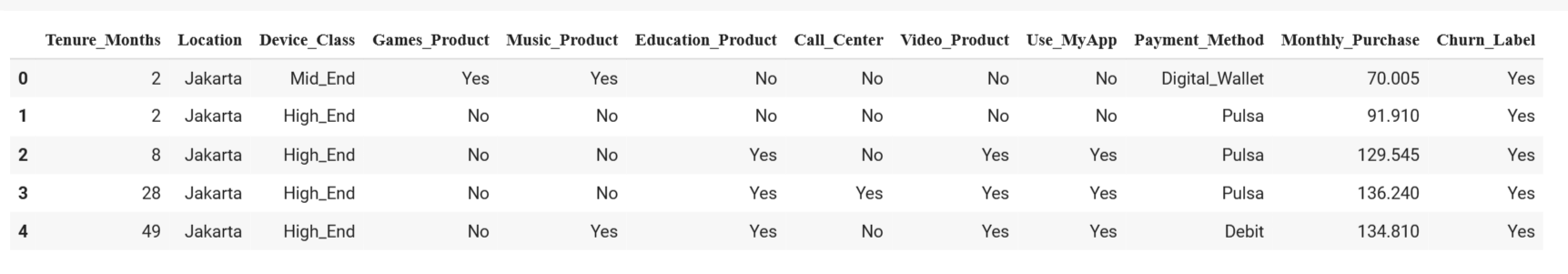
The dataset consists of 7043 rows, each representing a unique customer, and includes 14 features and 1 target feature (Churn). The data includes both numerical and categorical features, which will be addressed separately.

Target:

• Churn Label (Whether the customer left the company within a time period)

Numeric Features:

• Tenure Months (How long the customer has been with the company by the end of the quarter specified above)
• Monthly Purchase (Total customer’s monthly spent for all services with the unit of thousands of IDR)

Categorical Features:

• Customer ID (A unique customer identifier)
• Location (Customer’s residence - City)
• Device Class (Device classification)
• Games Product (Whether the customer uses the internet service for games product)
• Music Product (Whether the customer uses the internet service for music product)
• Education Product (Whether the customer uses the internet service for education product)
• Call Center (Whether the customer uses the call center service)
• Video Product (Whether the customer uses video product service)
• Use MyApp (Whether the customer uses MyApp service)
• Payment Method (The method used for paying the bill)

Churn Classification

Data Preparation

To facilitate the analytical process, i removed features such as CLTV, CustomerID, Latitude, and Longitude as they were not deemed pertinent for the analysis. I also made minor adjustments to the naming.

Feature Encoding

• One_hot_encoding will do for the nominal data: we cannot Rank the data, Example like zip-code
• Lavel_encoding we do for ordinal data : we can give a rank , example like Grade, education status

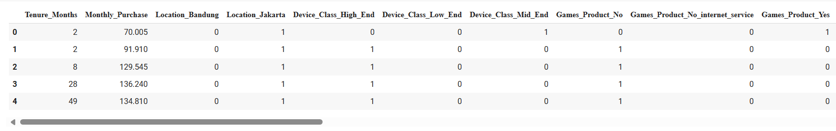
We are utilizing one-hot encoding because machine learning algorithms solely comprehend numerical data. Given that some of our predictors are categorical, we will employ the ‘get_dummies()’ function.

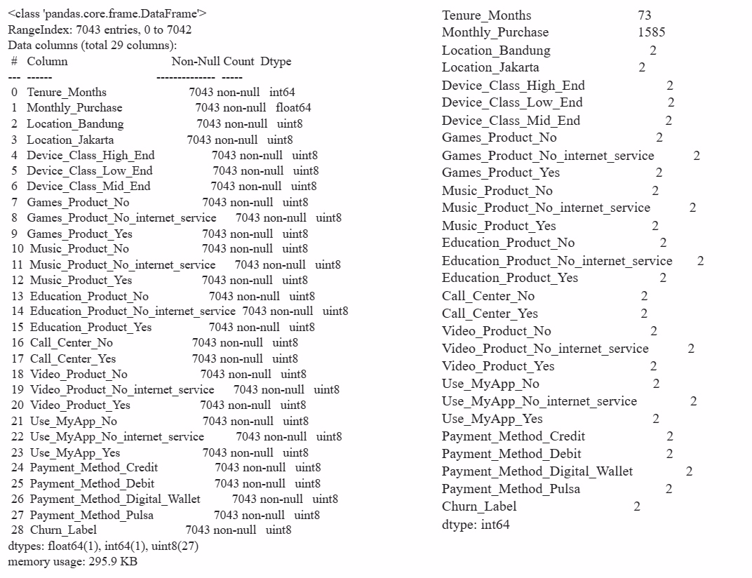
One hot coding is a technique that converts categorical variables into a binary representation, where each category is represented by a vector where only one element is 1 (hot) and the rest are 0 (cold). For example, for a location variable with the values Bandung and Jakarta, it would become two new variables: Bandung and Jakarta, where each would be 1 if the location matches and 0 if it does not, and this applies to other variables as well.

Split data and resample with SMOTE

over = SMOTE(sampling_strategy = 1)
x,y = over.fit_resample(x,y)
x_train, x_test, y_train, y_test = train_test_split(x, y, random_state =2, 
    test_size = 0.2)

The data is split into an 80:20 ratio and resampled using SMOTE to balance the class distribution in the dataset. This ensures that the model can learn patterns from both classes optimally.

Modelling

Comparative Analysis of Classification Models for Churn Prediction

def model(method, x_train, y_train, x_test, y_test):
    # Train the model
    method.fit(x_train, y_train)

    # Make predictions on test data and calculate confusion matrix
    predictions = method.predict(x_test)
    rmse = np.sqrt(mean_squared_error(y_test, predictions))
    c_matrix = confusion_matrix(y_test, predictions)

    # Calculate label percentages and create label strings with counts and percentages
    percentages = (c_matrix / np.sum(c_matrix, axis=1)[:, np.newaxis]).round(2) * 100
    labels = [[f"{c_matrix[i, j]} ({percentages[i, j]:.2f}%)" for j in range(c_matrix.shape[1])] for i in range(c_matrix.shape[0])]
    labels = np.asarray(labels)

    # Plot confusion matrix with labeled counts and percentages
    sns.heatmap(c_matrix, annot=labels, fmt='', cmap='Blues')

    # Evaluate model performance and print results
    print("RMSE:", rmse)
    print("ROC AUC: ", '{:.2%}'.format(roc_auc_score(y_test, predictions)))
    print("Model accuracy: ", '{:.2%}'.format(accuracy_score(y_test, predictions)))
    print(classification_report(y_test, predictions))
 
# Algorithm Model
xgb = XGBClassifier()
rf = RandomForestClassifier()
dt = DecisionTreeClassifier()

The reason for selecting XGBoost, Random Forest, and Decision Tree for churn classification is the combination of their respective strengths. XGBoost is chosen for its high performance, regularization capabilities to mitigate the risk of overfitting, and scalability to handle large datasets. Random Forest and Decision Tree are chosen for their flexibility to handle both categorical and numerical data without complex preprocessing, good interpretability, especially with Decision Tree, and resilience to unusual data or outliers. This combination allows us to leverage the strengths of each algorithm to build a robust and accurate churn classification model.

---

Result

XGBoost	Random Forest	Decision Tree
RMSE: 0.39440531887330776	RMSE: 0.40408541690413596	RMSE: 0.4493688542275248
ROC AUC: 84.44%	ROC AUC: 83.68%	ROC AUC: 79.81%
Model accuracy: 84.44%	Model accuracy: 83.67%	Model accuracy: 79.81%

XGBoost has an RMSE of 0.39440531887330776 and an ROC AUC of 84.44%, with a model accuracy of 84.44%. The RMSE and ROC AUC metrics for XGBoost, Random Forest, and Decision Tree models are as follows: Random Forest has an RMSE of 0. 40408541690413596 and an ROC AUC of 83.68%, with a model accuracy of 83.67%. Decision Tree has an RMSE of 0.4493688542275248 and an ROC AUC of 79.81%, with a model accuracy of 79.81%.

GridSearchCV for Optimal Parameters Comparative Classification Model Analysis

To enhance the model’s performance, we will conduct an optimal parameter search using GridsearchCV as the current results are suboptimal due to the Result Base Model. This will adjust the parameters to better fit the available data.

from sklearn.model_selection import GridSearchCV

# Define the parameter grid for each classifier
xgb_param_grid = {
    'learning_rate': [0.01, 0.1, 0.2],
    'max_depth': [3, 6, 9],
    'n_estimators': [500, 1000, 1500]
}

rf_param_grid = {	
    'n_estimators': [100, 200, 300],
    'max_depth': [None, 10, 20]
}

dt_param_grid = {
    'max_depth': [5, 10, 15, 20]
}

# Define classifiers
xgb = XGBClassifier()
rf = RandomForestClassifier()
dt = DecisionTreeClassifier()

# Perform grid search with cross-validation
xgb_grid_search = GridSearchCV(xgb, xgb_param_grid, cv=5)
rf_grid_search = GridSearchCV(rf, rf_param_grid, cv=5)
dt_grid_search = GridSearchCV(dt, dt_param_grid, cv=5)

# Fit the models
xgb_grid_search.fit(x_train, y_train)
rf_grid_search.fit(x_train, y_train)
dt_grid_search.fit(x_train, y_train)

# Get the optimal parameters for each classifier
best_xgb_params = xgb_grid_search.best_params_
best_rf_params = rf_grid_search.best_params_
best_dt_params = dt_grid_search.best_params_

print("Best parameters for XGBoost:", best_xgb_params)
print("Best parameters for Random Forest:", best_rf_params)
print("Best parameters for Decision Tree:", best_dt_params)

# Algorithm Model with Optimal Parameter
xgbcv = XGBClassifier(learning_rate= 0.01,max_depth = 9,n_estimators = 500)
rfcv = RandomForestClassifier(max_depth=20, n_estimators=100)
dtcv = DecisionTreeClassifier(max_depth=10)

---

Result with GridSearchCV

XGBoost	Random Forest	Decision Tree
RMSE: 0.39194794093833063	RMSE: 0.3931785497463923	RMSE: 0.4295824284138405
ROC AUC: 84.66%	ROC AUC: 84.56%	ROC AUC: 81.59%
Model accuracy: 84.64%	Model accuracy: 84.54%	Model accuracy: 81.55%

When using GridSearchCV for modeling, XGBoost outperformed the base results by producing a lower RMSE value of 0.39194794093833063, a higher ROC AUC of 84.66%, and a slightly higher model accuracy of 84.64%. This suggests that the process of searching for optimal parameter values using GridSearchCV has significantly improved the performance of the XGBoost model.

Random Forest also showed some improvement in performance, although not as much as XGBoost. The Random Forest with GridSearchCV improved the model’s performance compared to the base results, with an RMSE of 0.3931785497463923, ROC AUC of 84.56%, and model accuracy of 84.54%.

However, the Decision Tree, while showing improvement from the base results, still had lower performance compared to XGBoost and Random Forest. The results show that the Decision Tree model may not be appropriate for this dataset, even with the use of GridSearchCV. The RMSE is 0.4295824284138405, ROC AUC is 81.59%, and model accuracy is 81.55%.

The model’s performance has been improved through parameter optimization, particularly in the case of XGBoost and to a slightly lesser extent in Random Forest. Selecting optimal parameters is crucial for maximizing the performance of machine learning models.

Conclusions & Recommendations

Conclusion:

1. Customer churn analysis is a crucial step for companies, particularly in SaaS platforms, to comprehend customer behavior and anticipate potential churn.
2. Prior to building a classification model to predict customer churn, it is necessary to conduct exploratory data analysis (EDA) to gain a better understanding of the data.
3. After parameter selection using GridSearchCV, the XGBoost model demonstrated superior performance compared to Random Forest and Decision Tree.
4. After parameter tuning, XGBoost outperformed Random Forest in terms of lower RMSE, higher ROC AUC, and slightly higher model accuracy.
5. Although Random Forest also showed improvement, it was not as significant as XGBoost.
6. Even after using GridSearchCV, Decision Tree exhibited lower performance compared to XGBoost and Random Forest.
7. It is crucial to optimize parameters to maximize the performance of machine learning models.

Recommendations:

1. The company should continue using the XGBoost model to predict customer churn because of its superior performance.
2. It is important to monitor and evaluate model performance regularly to adjust business strategies accordingly.
3. Invest time and resources in comprehensive exploratory data analysis (EDA) before building models to ensure a better understanding of the data.
4. Use parameter tuning techniques, such as GridSearchCV, to significantly enhance model performance.
5. Continuously evaluate other models and consider upgrading or replacing them as necessary.
6. Additionally, integrate insights from this predictive model into the company’s customer retention strategy.

Thank you for completing the Telco Churn analysis with me. I hope the results are beneficial to you. Thanks for your participation!